Open an interactive online version by clicking the badge or download the notebook.

Overview of filters

The pyfar.dsp.filter module contains different filter types that are briefly introduced in the following. The filters can be used to directly filter pyfar Signals or can return a pyfar Filter object. For more information on this refer to the example notebooks on filtering and audio objects. All examples use an impulse to illustrate the different filter types.

import pyfar as pf
import matplotlib.pyplot as plt
%matplotlib inline

impulse = pf.signals.impulse(44100)

Standard filters

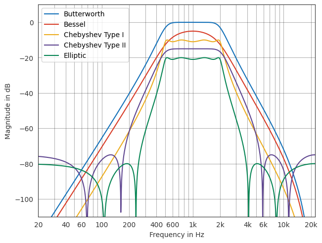
These are the classic filters that are wrapped from scipy.signal and available from the functions pyfar.dsp.filter.butterworth, pyfar.dsp.filter.bessel, pyfar.dsp.filter.chebyshev1, pyfar.dsp.filter.chebyshev2, and pyfar.dsp.filter.elliptic. They can be realized as high-pass, low-pass, band-pass, and band-stop filters as illustrated in the following examples.

High-pass filters

# filter order, cut-off frequency and type
N = 4
frequency = 1e3
btype = 'highpass'

# plot
y = pf.dsp.filter.butterworth(impulse, N, frequency, btype=btype)
ax = pf.plot.freq(y, label='Butterworth')

y = pf.dsp.filter.bessel(impulse, N, frequency, btype=btype)
pf.plot.freq(y * 10**(-5/20), label='Bessel')

y = pf.dsp.filter.chebyshev1(impulse, N, 1, frequency, btype=btype)
pf.plot.freq(y * 10**(-10/20), label='Chebyshev Type I')

y = pf.dsp.filter.chebyshev2(impulse, N, 60, 300, btype=btype)
pf.plot.freq(y * 10**(-15/20), label='Chebyshev Type II')

y = pf.dsp.filter.elliptic(impulse, N, 1, 60, frequency, btype=btype)
pf.plot.freq(y * 10**(-20/20), label='Elliptic')

ax.legend(loc='lower right');

Low-pass filters

btype = 'lowpass'

y = pf.dsp.filter.butterworth(impulse, N, frequency, btype=btype)
ax = pf.plot.freq(y, label='Butterworth')

y = pf.dsp.filter.bessel(impulse, N, frequency, btype=btype)
pf.plot.freq(y * 10**(-5/20), label='Bessel')

y = pf.dsp.filter.chebyshev1(impulse, N, 1, frequency, btype=btype)
pf.plot.freq(y * 10**(-10/20), label='Chebyshev Type I')

y = pf.dsp.filter.chebyshev2(impulse, N, 60, 3500, btype=btype)
pf.plot.freq(y * 10**(-15/20), label='Chebyshev Type II')

y = pf.dsp.filter.elliptic(impulse, N, 1, 60, frequency, btype=btype)
pf.plot.freq(y * 10**(-20/20), label='Elliptic')

ax.legend(loc='lower left');

Band-pass filters

frequency = [500, 2e3]
btype = 'bandpass'

y = pf.dsp.filter.butterworth(impulse, N, frequency, btype=btype)
ax = pf.plot.freq(y, label='Butterworth')

y = pf.dsp.filter.bessel(impulse, N, frequency, btype=btype)
pf.plot.freq(y * 10**(-5/20), label='Bessel')

y = pf.dsp.filter.chebyshev1(impulse, N, 1, frequency, btype=btype)
pf.plot.freq(y * 10**(-10/20), label='Chebyshev Type I')

y = pf.dsp.filter.chebyshev2(impulse, N, 60, [175, 5500], btype=btype)
pf.plot.freq(y * 10**(-15/20), label='Chebyshev Type II')

y = pf.dsp.filter.elliptic(impulse, N, 1, 60, frequency, btype=btype)
pf.plot.freq(y * 10**(-20/20), label='Elliptic')

ax.legend();

Band-stop filters

frequency = [250, 5e3]
btype = 'bandstop'

y = pf.dsp.filter.butterworth(impulse, N, frequency, btype=btype)
ax = pf.plot.freq(y, label='Butterworth')

y = pf.dsp.filter.bessel(impulse, N, frequency, btype=btype)
pf.plot.freq(y * 10**(-5/20), label='Bessel')

y = pf.dsp.filter.chebyshev1(impulse, N, 1, frequency, btype=btype)
pf.plot.freq(y * 10**(-10/20), label='Chebyshev Type I')

y = pf.dsp.filter.chebyshev2(impulse, N, 60, [175, 5500], btype=btype)
pf.plot.freq(y * 10**(-15/20), label='Chebyshev Type II')

y = pf.dsp.filter.elliptic(impulse, N, 1, 60, frequency, btype=btype)
pf.plot.freq(y * 10**(-20/20), label='Elliptic')

ax.legend(loc='lower left');

Linkwitz-Riley cross-over

The function pyfar.dsp.filter.crossover implements Linkwitz-Riley cross-over filters that are often used in loudspeaker design. The magnitude of the filters at the cross-over frequency is -6 dB and because the filters are in phase, their output adds to a constant magnitude response.

frequency = 1e3

y = pf.dsp.filter.crossover(impulse, N, frequency)
ax = pf.plot.freq(y, label=['low-pass', 'high-pass'])
pf.plot.freq(y[0] + y[1], color=[0, 0, 0, .5], linestyle='--', label='sum')

ax.legend(loc='lower left');

Filter banks

Filter banks are commonly used in audio and acoustics signal processing and pyfar contains the following filter banks.

Fractional octaves

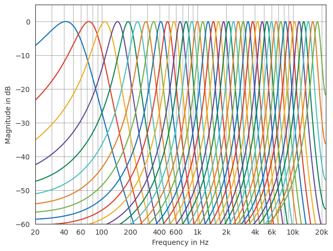
The fractional octave filter bank implemented in pyfar.dsp.filter.fractional_octave_bands is often used for calculating room acoustic parameters. The magnitude responses at the cut-off frequencies are -3 dB and hence the filter bank is approximately energy preserving.

y = pf.dsp.filter.fractional_octave_bands(impulse, 1, freq_range=(60, 12e3))
ax = pf.plot.freq(y)
ax.set_ylim(-60, 5);

The center frequencies of the filters are accessible via pyfar.dsp.filter.fractional_octave_frequencies.

Reconstructing fractional octaves

The reconstructing fractional octave filter bank implemented in pyfar.dsp.filter.reconstructing_fractional_octave_bands has -6 dB cut off frequencies and a linear phase response. This makes sure that any input can be perfectly reconstructed by summing the input, at the cost of adding a frequency independent delay of half the filter length. This filter bank can for example be used for room acoustical simulations.

y, *_ = pf.dsp.filter.reconstructing_fractional_octave_bands(impulse, 1)
ax = pf.plot.freq(y)
ax.set_ylim(-60, 5);

The center frequencies of the filters are accessible via pyfar.dsp.filter.fractional_octave_frequencies.

Gammatone (auditory)

The auditory gammatone filter bank implemented in pyfar.dsp.filter.GammatoneBands mimics the frequency selectivity of the human auditory system. It is almost perfectly reconstructing and is often used for binaural modeling. It is a direct port of the famous Hohmann2002 filter bank from the auditory modeling toolbox.

gtf = pf.dsp.filter.GammatoneBands((20, 20e3))
y, _ = gtf.process(impulse)
ax = pf.plot.freq(y)
ax.set_ylim(-60, 5);

The center frequencies of the filters are accessible via pyfar.dsp.filter.erb_frequencies.

Parametric equalizer

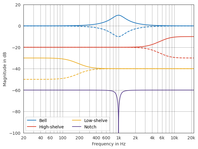
Parametric equalizers are specific filters used for example for audio effects or loudspeaker and room equalization. The bell filters implemented in pyfar.dsp.filter.bell manipulate the magnitude response around a center-frequency. The shelve filters implemented in pyfar.dsp.filter.high_shelve and pyfar.dsp.filter.low_shelve manipulate the magnitude response below or above a given characteristic frequency and the notch filters implemented in pyfar.dsp.filter.notch are very narrow band rejection filters.

y = pf.dsp.filter.bell(impulse, frequency, 10, 2)
ax = pf.plot.freq(y, label='Bell')

y = pf.dsp.filter.bell(impulse, frequency, -10, 2)
pf.plot.freq(y, color='b', linestyle='--')

y = pf.dsp.filter.high_shelve(impulse, 4*frequency, 10, 2, 'II')
pf.plot.freq(y * 10**(-20/20), label='High-shelve')

y = pf.dsp.filter.high_shelve(impulse, 4*frequency, -10, 2, 'II')
pf.plot.freq(y * 10**(-20/20), color='r', linestyle='--')

y = pf.dsp.filter.low_shelve(impulse, 1/4*frequency, 10, 2, 'II')
pf.plot.freq(y * 10**(-40/20), label='Low-shelve')

y = pf.dsp.filter.low_shelve(impulse, 1/4*frequency, -10, 2, 'II')
pf.plot.freq(y * 10**(-40/20), color='y', linestyle='--')

y = pf.dsp.filter.notch(impulse * .1**3, 1000, 4)
pf.plot.freq(y, label='Notch')

ax.set_ylim(-100, 20)
ax.legend(loc='lower left', ncol=2);

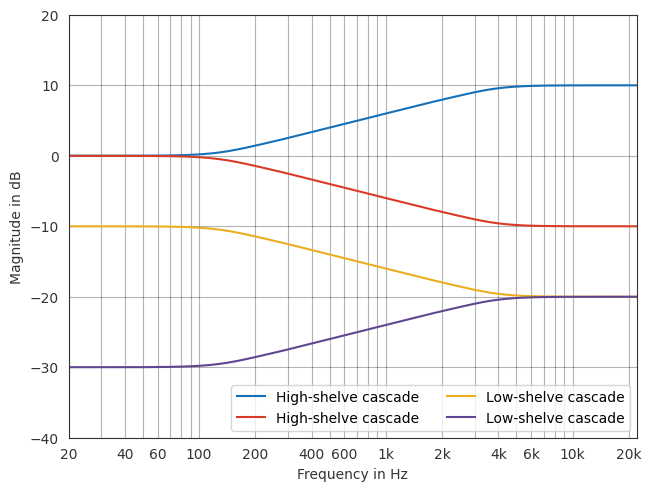
The cascaded shelving filters implemented in pyfar.dsp.filter.low_shelve_cascade and pyfar.dsp.filter.high_shelve_cascade shown on the right can be used to generate filters with a user definable slope given in dB per octaves within a certain frequency region. They are also termed High-Schultz and Low-Shultz filters to acknowledge one of their inventors Frank Schultz.

y, *_ = pf.dsp.filter.high_shelve_cascade(impulse, 125, 'lower', 10, None, 5)
ax = pf.plot.freq(y, label="High-shelve cascade")

y, *_ = pf.dsp.filter.high_shelve_cascade(impulse, 125, 'lower', -10, None, 5)
pf.plot.freq(y, label="High-shelve cascade")

y, *_ = pf.dsp.filter.low_shelve_cascade(impulse, 125, 'lower', 10, None, 5)
pf.plot.freq(y * 10**(-20/20), label="Low-shelve cascade")

y, *_ = pf.dsp.filter.low_shelve_cascade(impulse, 125, 'lower', -10, None, 5)
pf.plot.freq(y * 10**(-20/20), label="Low-shelve cascade")

ax.set_ylim(-40, 20)
ax.legend(loc='lower right', ncol=2);

License notice

This notebook © 2024 by the pyfar developers is licensed under CC BY 4.0

Watermark

%load_ext watermark
%watermark -v -m -iv

Python implementation: CPython
Python version       : 3.10.13
IPython version      : 8.23.0

Compiler    : GCC 11.4.0
OS          : Linux
Release     : 5.19.0-1028-aws
Machine     : x86_64
Processor   : x86_64
CPU cores   : 2
Architecture: 64bit

matplotlib: 3.7.0
pyfar     : 0.6.5