
Coordinates#
In acoustics research, we often deal with different coordinate systems when handling sampling points, for example, microphone positions in a spherical microphone array or loudspeaker positions in a sound field synthesis system. This can get complicated. That’s why we have the pyfar.Coordinates . The class was designed for storing, working with, and accessing coordinate points. You can easily switch between different coordinate systems, rotate points, and do other useful operations.
[1]:
import pyfar as pf
import numpy as np
%matplotlib inline
Supported Coordinate systems#
Common coordinate systems are the cartesian, spherical and cylindrical systems, where different conventions exist for spherical coordinates. A coordinate system is defined by a set of coordinates, e.g. cartesian consists of the coordinates x, y, and z. Please have a look on the documentation, you will find a figure with all coordinate systems definitions.
Note that each coordinate has a unique name. If a coordinate is contained in multiple coordinate systems (e.g. ‘z’ in cartesian and cylindrical) this means the values for z are the same in both cases.
Entering points#
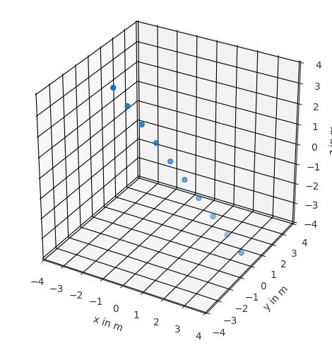
You can input points manually into the system. By default, the system assumes cartesian coordinates.
[2]:
# create a coordinates object with x values from -5 to 5 any y and z values 0
c = pf.Coordinates(np.arange(-5, 6), 0, 0)
# plot the sampling points
c.show()
[2]:
<Axes3D: xlabel='x in m', ylabel='y in m', zlabel='z in m'>

To initialize Coordinates objects for different coordinate systems, you can use specific constructors like pf.Coordinates.from_spherical_elevation(azimuth, elevation, radius). The naming convention for these constructors is always pf.Coordinates.from_coordinate_system(red, green, blue), where coordinate_system should be replaced with the desired coordinate system, and red, green, blue describe the order of the coordinate properties. The colors and the
coordinate_system names can be found in the figure above. Remember, angles are always defined in radians.
For more details, you can refer to the coordinate class documentation.
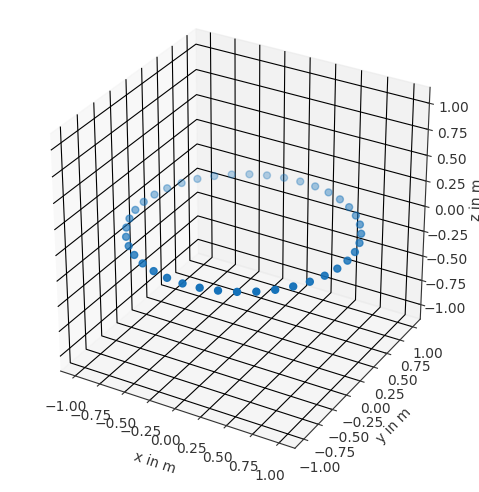
[3]:
azimuth_angles = np.arange(0, 2*np.pi, np.pi/20)
c1 = pf.Coordinates.from_spherical_elevation(azimuth_angles, 0, 1)
c1.show()
[3]:
<Axes3D: xlabel='x in m', ylabel='y in m', zlabel='z in m'>
Meta data#
In addition to the data points, coordinate objects also store meta data. Lets have a look by printing the coordinate object.
[4]:
print(c1)
1D Coordinates object with 40 points of cshape (40,)

Does not contain sampling weights
We can observe that there are 40 coordinate points in the object. This refers to the attribute coordinate size or in short csize.
[5]:
c1.csize
[5]:
40
The coordinate shape or in short cshape of the data is (40,) and specifies how the 40 coordinate points are organized. In this case they are organized in a single dimension, but Coordinates of csize = 40 could for example also be organized in a cshape = (2, 20) because the csize is the product of the cshape.
[6]:
c1.cshape
[6]:
(40,)
Similarly, cdim returns the number of dimensions of the coordinate points, which is given by the length of the cshape and is 1 in this case.
[7]:
c1.cdim
[7]:
1
The cshape, csize, and cdim attributes are similar to the pyfar Audio classes.
Retrieving coordinate points#
There are different ways to retrieve points from a Coordinates object. All points can be obtained in cartesian, spherical, and cylindrical coordinates using the related properties c.cartesian, c.sperical_evaluation and c.cylindrical. Visit the coordinate class for more details.
[8]:
# access cartesian coordinates x, y, z
c.cartesian
[8]:
array([[-5.,  0.,  0.],
       [-4.,  0.,  0.],
       [-3.,  0.,  0.],
       [-2.,  0.,  0.],
       [-1.,  0.,  0.],
       [ 0.,  0.,  0.],
       [ 1.,  0.,  0.],
       [ 2.,  0.,  0.],
       [ 3.,  0.,  0.],
       [ 4.,  0.,  0.],
       [ 5.,  0.,  0.]])
We use Cartesian coordinates to store points internally. If you input points in a different coordinate system, we convert them to Cartesian coordinates before saving them. Similarly, if you request data in a different coordinate system, we convert it on the spot. Sometimes, these conversions can result in tiny numerical inaccuracies, typically around \(10^{-16}\).
[9]:
# access spherical coordinates azimuth, elevation, radius
c.spherical_elevation
[9]:
array([[3.14159265, 0.        , 5.        ],
       [3.14159265, 0.        , 4.        ],
       [3.14159265, 0.        , 3.        ],
       [3.14159265, 0.        , 2.        ],
       [3.14159265, 0.        , 1.        ],
       [0.        , 0.        , 0.        ],
       [0.        , 0.        , 1.        ],
       [0.        , 0.        , 2.        ],
       [0.        , 0.        , 3.        ],
       [0.        , 0.        , 4.        ],
       [0.        , 0.        , 5.        ]])
Note that angles are always returned in radian. We can convert from radian to degree by using pyfar.rad2deg.
[10]:
spherical_elevation_deg = pf.rad2deg(c.spherical_elevation)
spherical_elevation_deg
[10]:
array([[180.,   0.,   5.],
       [180.,   0.,   4.],
       [180.,   0.,   3.],
       [180.,   0.,   2.],
       [180.,   0.,   1.],
       [  0.,   0.,   0.],
       [  0.,   0.,   1.],
       [  0.,   0.,   2.],
       [  0.,   0.,   3.],
       [  0.,   0.,   4.],
       [  0.,   0.,   5.]])
Or vice versa using pyfar.deg2rad.
[11]:
spherical_elevation_rad = pf.deg2rad(spherical_elevation_deg)
spherical_elevation_rad
[11]:
array([[3.14159265, 0.        , 5.        ],
       [3.14159265, 0.        , 4.        ],
       [3.14159265, 0.        , 3.        ],
       [3.14159265, 0.        , 2.        ],
       [3.14159265, 0.        , 1.        ],
       [0.        , 0.        , 0.        ],
       [0.        , 0.        , 1.        ],
       [0.        , 0.        , 2.        ],
       [0.        , 0.        , 3.        ],
       [0.        , 0.        , 4.        ],
       [0.        , 0.        , 5.        ]])
ALso, single properties of all implemented coordinate system conventions can be accessed, e.g. azimuth, radius or x. The shape of these numpy arrays equals the cshape of the Coordinates object.
[12]:
c.azimuth
[12]:
array([3.14159265, 3.14159265, 3.14159265, 3.14159265, 3.14159265,
       0.        , 0.        , 0.        , 0.        , 0.        ,
       0.        ])
Manipulating points#
the previous attributes can also be used to manipualte the data.
[13]:
azimuth = c.azimuth
azimuth[0] = 0
c.azimuth = azimuth
c.azimuth
[13]:
array([0.        , 3.14159265, 3.14159265, 3.14159265, 3.14159265,
       0.        , 0.        , 0.        , 0.        , 0.        ,
       0.        ])
Accessing subsets#
Different methods are available for obtaining a specific subset of coordinates.
Find nearest#
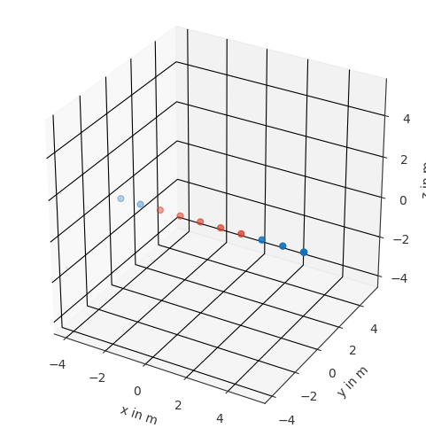
The first method is to find the subset of nearest points to a given point.
[14]:
# find nearest points to x=0, y=-1, z=0
p = pf.Coordinates.from_cartesian(0, -1, 0)
index_out, distance = c.find_nearest(p)
c.show(index_out)
[14]:
<Axes3D: xlabel='x in m', ylabel='y in m', zlabel='z in m'>

If we want to find the nearest 3 points, then we need to set k=3.
[15]:
index_out, distance = c.find_nearest(p, k=3)
c.show([index_out[0], index_out[1], index_out[2]])
[15]:
<Axes3D: xlabel='x in m', ylabel='y in m', zlabel='z in m'>

Note that the distance to the finding points is also returned.
[16]:
distance
[16]:
array([1. , 1.41421356, 1.41421356])
Of course you can also get a copy of the points, if want to continue working just with the subset.
[17]:
p_1 = c[index_out[1]]
p_1
[17]:
1D Coordinates object with 1 points of cshape (1,)

Does not contain sampling weights
Find within#
Another option is to find all points within a certain distance. Different distance measures are available, see the pyfar documentation for more information.
[18]:
# Find all points within a distance of 3 from the point find
index_out = c.find_within(p, distance=3, distance_measure='euclidean')
c.show(index_out)
[18]:
<Axes3D: xlabel='x in m', ylabel='y in m', zlabel='z in m'>
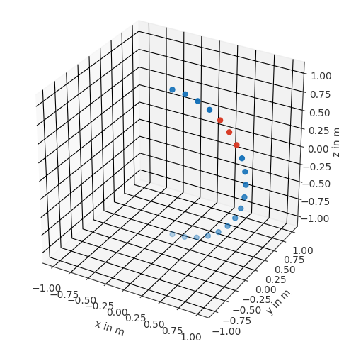
Logical operations with attributes#
Another way is to apply logical operations directly to the coordinate attributes. As an example, we create a half arc. Then to obtain all points within a between 30° and 60° elevation, we just need to apply logical operations as follows.
[19]:
c2 = pf.Coordinates.from_spherical_colatitude(0, np.arange(0, 181, 10)*np.pi/180, 1)
index_out = (c2.elevation*180/np.pi >= 30) & (c2.elevation*180/np.pi <= 60)
c2.show(np.where(index_out))
[19]:
<Axes3D: xlabel='x in m', ylabel='y in m', zlabel='z in m'>
Rotating coordinates#
You can apply rotations using quaternions, rotation vectors/matrixes and euler angles with c.rotate(), which is a wrapper for scipy.spatial.transform.Rotation. For example, rotating around the y-axis by 45 degrees can be done with
[20]:
c.rotate('y', 45)
c.show()
[20]:
<Axes3D: xlabel='x in m', ylabel='y in m', zlabel='z in m'>
Note that this changes the points inside the Coordinates object, which means that you have to be careful not to apply the rotation multiple times, i.e., when evaluationg cells during debugging.
License notice#
This notebook © 2024 by the pyfar developers is licensed under CC BY 4.0

Watermark#
[21]:
%load_ext watermark
%watermark -v -m -iv
Python implementation: CPython
Python version       : 3.13.3
IPython version      : 9.13.0

Compiler    : GCC 11.4.0
OS          : Linux
Release     : 6.17.0-1007-aws
Machine     : x86_64
Processor   : x86_64
CPU cores   : 2
Architecture: 64bit

numpy: 2.4.4
pyfar: 0.8.0