Open an interactive online version by clicking the badge or download the notebook.

Fast Fourier Transform (FFT)

The following gives background information that is helpful to understand how the Fast Fourier Transform (FFT) and the corresponding normalizations are defined in pyfar and how these are related to the concepts of energy and power signals.

FFT definition

The discrete Fourier transform (DFT) of an arbitrary, but band-limited signal \(x(n)\) is defined as

\[X(k) = \sum_{n=0}^{N-1} x(n) e^{-i 2 \pi k \frac{n}{N}}\]

using a negative sign convention in the transform kernel \(e^{-i 2 \pi k \frac{n}{N}}\), and normalized angular frequency \(\omega_k = 2 \pi k / N\). Analogously, the inverse discrete Fourier transform (IDFT) is defined as

\[x(n) = \frac{1}{N} \sum_{k=0}^{N-1} X(k) e^{i2\pi k \frac{n}{N}}\]

The Fast Fourier Transform denotes the efficient implementation of the DFT and IDFT.

Note that real-valued time signals result in Fourier spectra with complex conjugate symmetry for negative and positive frequencies \(X(k) = X(-k)^*\). In this case, the left-hand side of the spectrum can be discarded, and only the right-hand side needs to be saved.

FFT normalizations

Pyfar implements five normalizations after Ahrens at al. (2020) that can be applied to spectra after the DFT. The normalizations are implicitly used by the pyfar.Signal class, and are available from pyfar.dsp.fft.normalization. For a Signal object signal, signal.freq contains the normalized spectrum according to signal.fft_norm and signal.freq_raw contains the raw spectrum without any normalization. The time data (signal.time) does not change regardless of the normalization.

The following table shows the available normalizations and their definitions:

Normalization	Equation
'none'	–
'unitary'	\(X_{\text{SS}}(k) = \left\{ \begin{array}{ll} X(k) & \forall k=0, k=\frac{N}{2} \\ 2 X(k) & \forall 0<k< \frac{N}{2} \end{array} \right.\)
'amplitude'	\(\overline{X}_{\text{SS}}(k) = \frac{1}{N} X_{\text{SS}}(k)\)
'rms'	\(\overline{X}_{RMS}(k) = \left\{ \begin{array}{ll} \frac{1}{\sqrt{2}} \overline{X}_{\text{SS}}(k) & \forall 0<k< \frac{N}{2} \\ \quad \overline{X}_{\text{SS}}(k) & \forall k=0, k=\frac{N}{2} \end{array} \right.\)
'power'	\(\overline{\overline{X}}_{\text{SS}}(k) = \lvert \overline{X}_{\text{RMS}}(k) \lvert ^2\)
'psd'	\(\overline{\overline{\underline{X}}}_{\text{SS}}(k) = \frac{N}{f_s} \overline{\overline{X}}_{\text{SS}}(k) = \frac{N}{f_s} \lvert \overline{X}_{\text{RMS}}(k) \lvert ^2\)

Note that the above formulation holds for real-valued signals with single-sided spectra \(X_{\text{SS}}(k)\). Hence, there are small differences in the definitions compared to the formulas written in Ahrens et al. (2020).

Example signals

Four signals with a length of 100 samples and a sampling rate of 10 kHz are used for illustrating the normalizations.

import pyfar as pf
import numpy as np
import matplotlib.pyplot as plt

%matplotlib inline

# set number of samples and sampling rate
n_samples = 1e3
sampling_rate = 10e3

An impulse (\(x(0)=1\) and zero otherwise) with a constant spectrum.

impulse = pf.signals.impulse(n_samples, sampling_rate=sampling_rate)

A fractional octave FIR filter presenting a system with finite energy (e.g., a loudspeaker transfer function, a room impulse response, an HRTF …).

fir = pf.dsp.filter.fractional_octave_bands(
    impulse, num_fractions=1, freq_range=(500, 700))

A sine signal with an amplitude of \(1\,\text{Pa}\). It represents a discrete tone of which a snippet was recorded.

sine = pf.signals.sine(1e3, n_samples, sampling_rate=sampling_rate)

A white noise signal with an RMS value of \(1/\sqrt{2}\,\text{Pa}\). It represents a broadband stochastic signal of which a snippet was recorded of.

noise = pf.signals.noise(
    n_samples, rms=1/np.sqrt(2), sampling_rate=sampling_rate)

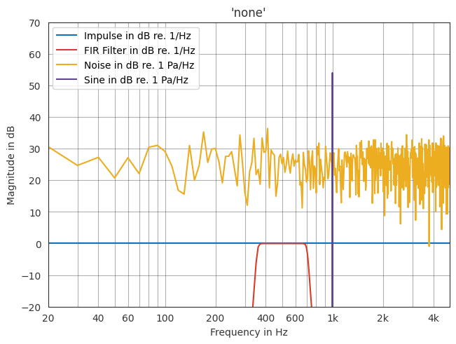
'none'

The 'none' normalization (the default) uses the FFT spectrum as it is. This norm is to be used for energy signals such as impulse responses, as illustrated below by the impulse and FIR filter. With this normalization, the spectrum is independent of the signal length. Yet, the spectrum depends on the number of samples for power signals, such as the sine and noise (“longer signal = more energy”). For example, the magnitude of the sine equals of number of samples/2 (1000/2, 60-6 dB). For that reason, other normalizations are appropriate for power signals.

for signal in [impulse, fir, sine, noise]:
    signal.fft_norm = 'none'

ax = pf.plot.freq(impulse, label="Impulse in dB re. 1/Hz")
pf.plot.freq(fir, label="FIR Filter in dB re. 1/Hz")
pf.plot.freq(noise, label="Noise in dB re. 1 Pa/Hz")
pf.plot.freq(sine, label="Sine in dB re. 1 Pa/Hz")

ax.set_title("'none'")
ax.set_ylim(-20, 70)
ax.legend(loc='upper left')

<matplotlib.legend.Legend at 0x7f0e5bf27ac0>

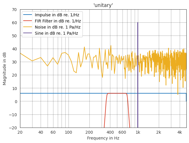
'unitary'

The FFT-calculated spectrum is multiplied by a factor of 2 in order to represent power related measures correctly. This results in +6 dB in magnitude in the plot below compared to the 'none'’ normalization. All following normalizations make use of this (implicitly assuming real-valued time signals, i.e., signals with single-sided spectrum).

for signal in [impulse, fir, sine, noise]:
    signal.fft_norm = 'unitary'

ax = pf.plot.freq(impulse, label="Impulse in dB re. 1/Hz")
pf.plot.freq(fir, label="FIR Filter in dB re. 1/Hz")
pf.plot.freq(noise, label="Noise in dB re. 1 Pa/Hz")
pf.plot.freq(sine, label="Sine in dB re. 1 Pa/Hz")

ax.set_title("'unitary'")
ax.set_ylim(-20, 70)
ax.legend(loc='upper left')

<matplotlib.legend.Legend at 0x7f0e599ffa30>

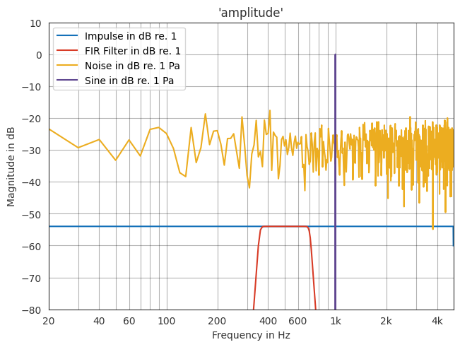
'amplitude'

The spectrum is normalized to show the amplitude of the pure tone components contained in a signal by considering the number of samples. Accordingly, the sine signal with an amplitude of 1 has an absolute value of 1 Pa (0 dB) at the frequency of the sine, with the implied unit “Pa” being illustrated correctly.

for signal in [impulse, fir, sine, noise]:
    signal.fft_norm = 'amplitude'

ax = pf.plot.freq(impulse, label="Impulse in dB re. 1")
pf.plot.freq(fir, label="FIR Filter in dB re. 1")
pf.plot.freq(noise, label="Noise in dB re. 1 Pa")
pf.plot.freq(sine, label="Sine in dB re. 1 Pa")

ax.set_title("'amplitude'")
ax.set_ylim(-80, 10)
ax.legend(loc='upper left')

<matplotlib.legend.Legend at 0x7f0e5875beb0>

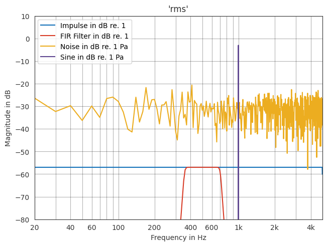
'rms'

The spectrum is normalized to show the RMS value of the pure tone components contained in a signal. This results in a magnitude of -3 dB re. 1 Pa of the sine.

for signal in [impulse, fir, sine, noise]:
    signal.fft_norm = 'rms'

ax = pf.plot.freq(impulse, label="Impulse in dB re. 1")
pf.plot.freq(fir, label="FIR Filter in dB re. 1")
pf.plot.freq(noise, label="Noise in dB re. 1 Pa")
pf.plot.freq(sine, label="Sine in dB re. 1 Pa")

ax.set_title("'rms'")
ax.set_ylim(-80, 10)
ax.legend(loc='upper left')

<matplotlib.legend.Legend at 0x7f0e58677d00>

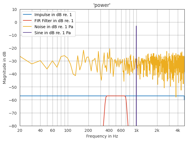
'power'

In a dB representation, 'power' normalization equals the 'rms' normalization, when correctly accounting for the prefix 10 in the dB calculation. Though meaningful for pure tones, these normalizations result in a dependence of the magnitude on the sampling rate for stochastic broadband signals such as the noise signal, as these are defined by a constant power density (see 'psd').

for signal in [impulse, fir, sine, noise]:
    signal.fft_norm = 'power'

ax = pf.plot.freq(impulse, log_prefix=10, label="Impulse in dB re. 1")
pf.plot.freq(fir, log_prefix=10, label="FIR Filter in dB re. 1")
pf.plot.freq(noise, log_prefix=10, label="Noise in dB re. 1 Pa")
pf.plot.freq(sine, log_prefix=10, label="Sine in dB re. 1 Pa")

ax.set_title("'power'")
ax.set_ylim(-80, 10)
ax.legend(loc='upper left')

<matplotlib.legend.Legend at 0x7f0e585d6470>

'psd'

Using 'psd' normalization, signals are represented as power densities (e.g. in Pa²/Hz), leading to a meaningful representation for broadband stochastic signals independently of the sampling rate. From the examples, this normalization is only meaningful for the noise signal. With this normalization, the sine’s magnitude is reduced by a factor of number of samples / sampling rate (1/10, -10 dB) compared to 'rms' and 'power'.

for signal in [impulse, fir, sine, noise]:
    signal.fft_norm = 'psd'

ax = pf.plot.freq(
    impulse, log_prefix=10, label="Impulse in dB re. 1/$\sqrt{\mathrm{Hz}}$")
pf.plot.freq(
    fir, log_prefix=10, label="FIR Filter in dB re. 1/$\sqrt{\mathrm{Hz}}$")
pf.plot.freq(
    noise, log_prefix=10, label="Noise in dB re. 1 Pa/$\sqrt{\mathrm{Hz}}$")
pf.plot.freq(
    sine, log_prefix=10, label="Sine in dB re. 1 Pa/$\sqrt{\mathrm{Hz}}$")

ax.set_title("'psd'")
ax.set_ylim(-80, 10)
ax.legend(loc='upper left')

<matplotlib.legend.Legend at 0x7f0e5830bbe0>

Summary

The table summarizes which normalization to use for which type of signal.

Signal type	Variation	Normalization
Energy	Impulse responses / transfer functions	'none'
Power	Discrete tones	'amplitude', 'rms', 'power'
Power	Broadband stochastic signals	'psd'

For further details, especially on the background of the power normalizations, it is referred to Ahrens at al. (2020). See pyfar.dsp.fft for a complete documentation.

Reference

J. Ahrens, C. Andersson, P. Höstmad, and W. Kropp, “Tutorial on Scaling of the Discrete Fourier Transform and the Implied Physical Units of the Spectra of Time-Discrete Signals,” AES Convention e-Brief 600, May 2020.

License notice

This notebook © 2024 by the pyfar developers is licensed under CC BY 4.0

Watermark

%load_ext watermark
%watermark -v -m -iv

Python implementation: CPython
Python version       : 3.10.13
IPython version      : 8.23.0

Compiler    : GCC 11.4.0
OS          : Linux
Release     : 5.19.0-1028-aws
Machine     : x86_64
Processor   : x86_64
CPU cores   : 2
Architecture: 64bit

matplotlib: 3.7.0
numpy     : 1.26.4
pyfar     : 0.6.5