Welcome#
The Python package for Acoustics Research (pyfar) contains classes and functions for the acquisition, inspection, and processing of audio signals. This is the pyfar demo notebook and a good place for getting started. In this notebook, you will see examples of the most important pyfar functionalty.
Note: This is not a substitute for the pyfar documentation that provides a complete description of the pyfar functionality.
Contents#
Getting started
Handling Audio Data - FFT normalization - Energy and power signals - Accessing Signal data - Iterating Signals - Signal meta data - Arithmetic operations - Plotting - Interactive plots - Manipulating plots
Coordinates - Entering coordinate points - Retrieving coordinate points - Rotating coordinate points
Orientations - Entering orientations - Retrieving orientations - Rotating orientations
DSP - Filtering
In’n’out - Read and write workspace - Read and write audio files - Read SOFA files
Lets start with importing pyfar and numpy:
Getting started#
Please note that this is not a Python tutorial. We assume that you are aware of basic Python coding and concepts including the use of conda and pip. If you did not install pyfar already please do so by running the command
pip install pyfar
After this go to your Python editor of choice and import pyfar
[1]:
# import packages
import pyfar as pf
import numpy as np

# set matplotlib backend for plotting
%matplotlib inline
Handling audio data#
Audio data are the basis of pyfar and there are three classes for storing and handling it. Most data will be stored in objects of the Signal class, which is intended for time and frequency data that was sampled at equidistant times and frequencies. Examples for this are audio recordings or single sided spectra between 0 Hz and half the sampling rate.
The other two classes TimeData and FrequencyData are intended to store inclomplete audio data. For example time signals that were not sampled at equidistant times or frequency data that are not available for all frequencies between 0 Hz and half the sampling rate. We will only look at Signals, however, TimeDataand FrequencyData are very similar.
Signals are stored along with information about the sampling rate, the domain (time, or freq), the FFT normalization and an optional comment. Lets go ahead and create a single channel signal
[2]:
# create a dirac signal with a sampling rate of 44.1 kHz
fs = 44100
x = np.zeros(44100)
x[0] = 1
x_energy = pf.Signal(x, fs)

# show information
x_energy
[2]:
time domain energy Signal:
(1,) channels with 44100 samples @ 44100 Hz sampling rate and none FFT normalization
FFT Normalization#
Different FFT normalization are available that scale the spectrum of a Signal. Pyfar knows six normalizations: 'amplitude', 'rms', 'power', and 'psd' from Ahrens, et al. 2020, 'unitary' (only applies weights for single sided spectra as in Eq. 8 in Ahrens, et al. 2020), and 'none' (applies no normalization). The default normalization is 'none', which is useful for
energy signals, i.e., signals with finite energy such as impulse responses. The other FFT normalizations are intended for power signals, i.e., samples of signals with infinite energy, such as noise or sine signals. Visit the FFT concepts for more information. Let’s create a signal with a different normalization
[3]:
x = np.sin(2 * np.pi * 1000 * np.arange(441) / fs)
x_power = pf.Signal(x, fs, fft_norm='rms')
x_power
[3]:
time domain power Signal:
(1,) channels with 441 samples @ 44100 Hz sampling rate and rms FFT normalization
The normalization can be changed. In this case the spectral data of the signal is converted internally using pyfar.fft.normalization()
[4]:
x_power.fft_norm = 'amplitude'
x_power
[4]:
time domain power Signal:
(1,) channels with 441 samples @ 44100 Hz sampling rate and amplitude FFT normalization
Note the following:
The normalizations are only relevant for inspecting the magnitude data, i.e., in plotting. pyfar thus uses the non normalized spectra for all signal processing and arithmetic operations.
FrequencyDataobjects do not support the FFT normalization because this requires knowledge about the sampling rate or the number of samples of the time signal. These objects thus have the'none'in all cases.TimeDatadoes not support FFT normalization because it only exists in the time domain. These objects do not have thefft_normattribute at all.
Energy and power signals#
You might have realized that pyfar distinguishes between energy and power signals, which is required for some operations. Signals with the FFT normalization 'none' are considered as energy signals while all other FFT normalizations result in power signals.
Accessing Signal data#
You can access the data, i.e., the audio signal, inside a Signal object in the time and frequency domain by simply using
[5]:
time_data = x_power.time
freq_data_normalized = x_power.freq
freq_data_raw = x_power.freq_raw
Two things are important here:
The data are mutable! That means
x_power.timechanges if you changetime_data. If this is not what you want usetime_data = x_power.time.copy()instead.The frequency data of signals is available without normalization from
x_power.freq_rawand with normalization fromx_power.freq. The latter depends on the Signal’sfft_norm.
Signals and some other pyfar objects support slicing. Let’s illustrate that for a two channel signal
[6]:
# generate two channel time data
time = np.zeros((2, 4))
time[0,0] = 1   # first sample of first channel
time[1,0] = 2   # first sample of second channel

x_two_channels = pf.Signal(time, 44100)
x_first_channel = x_two_channels[0]
x_first_channel is a Signal object itself, which contains the first channel of x_two_channels:
[7]:
x_first_channel.time
[7]:
array([[1., 0., 0., 0.]])
A third option to access Signals is to copy it
[8]:
x_copy = x_two_channels.copy()
It is important to note that this returns an independent copy of x_two_channels. Note that x_copy = x_two_channels might not be wanted. In this case changes to x_copy will also change x_two_channels. The copy() operation is available for all pyfar objects.
Iterating Signals#
It is the aim of pyfar that all operations work on N-dimensional signals. Nevertheless, you can also iterate signals if you need to apply operations depending on the channel. Lets look at a simple example
[9]:
signal = pf.Signal([[0, 0, 0], [1, 1, 1]], 44100)  # 2-channel signal

# iterate the signal
for n, channel in enumerate(signal):
    print(f"Channel: {n}, time data: {channel.time}")
    # do something channel dependent
    channel.time = channel.time + n
    # write changes to the signal
    signal[n] = channel

# q.e.d.
print(f"\nNew signal time data:\n{signal.time}")
Channel: 0, time data: [[0. 0. 0.]]
Channel: 1, time data: [[1. 1. 1.]]

New signal time data:
[[0. 0. 0.]
 [2. 2. 2.]]
Signal uses the standard numpy iterator which always iterates the first dimension. In case of a 2-D array as in the example above these are the channels.
Signal meta data#
The Signal object also holds useful metadata. The most important might be:
Signal.n_samples: The number of samples in each channel (Signal.time.shape[-1])Signal.n_bins: The number of frequencies in each channel (Signal.freq.shape[-1])Signal.times: The sampling times ofSignal.timein secondsSignal.frequencies: The frequencies ofSignal.freqin HzSignal.comment: A comment for documenting the signal content
Arithmetic operations#
The arithmetic operations add, subtract, multiply, divide, and power are available for Signal (time or frequency domain operations) as well as for TimeData and FrequencyData. The operations work on arbitrary numbers of Signals and array likes. Lets check out simple examples
[10]:
# add two signals energy signals
x_sum = pf.add((x_energy, x_energy), 'time')
x_sum.time
[10]:
array([[2., 0., 0., ..., 0., 0., 0.]])
In this case, x_sum is also an energy Signal. However, this can be different for other operation as described in the documentation (arithmetic operations). Under the hood, the operations use numpy’s array broadcasting. This means you can add scalars, vectors, and matrixes to a signal. Lets
have a frequency domain example for this
[11]:
x_sum = pf.add((x_energy, 1), 'freq')
x_sum.time
[11]:
array([[2., 0., 0., ..., 0., 0., 0.]])
The Python operators +, -, *, /, ** and @ are overloaded with the frequency domain arithmetic functions for Signal and FrequencyData. For TimeData they correspond to time domain operations. Thus, the example above can also be shortened to
[12]:
x_sum = x_energy + 1
x_sum.time
[12]:
array([[2., 0., 0., ..., 0., 0., 0.]])
Plotting#
Inspecting signals can be done with the pyfar.plot module, which uses common plot functions based on Matplotlib. For example a plot of the magnitude spectrum
[13]:
pf.plot.freq(x_power)
[13]:
<Axes: xlabel='Frequency in Hz', ylabel='Magnitude in dB'>
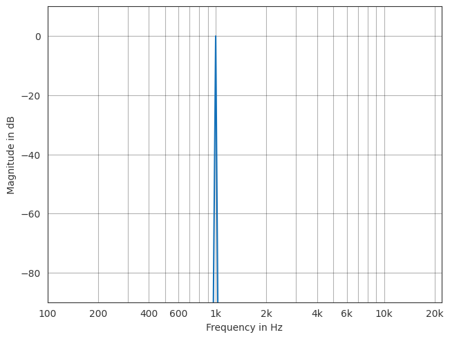
We set the FFT normalization to ‘amplitude’ before. The plot thus shows the amplitude (1, or 0 dB) of our sine wave contained in x_power. We can also plot the RMS (\(1/\sqrt(2)\), or \(\approx-3\) dB)
[14]:
x_power.fft_norm = 'rms'
pf.plot.line.freq(x_power)
[14]:
<Axes: xlabel='Frequency in Hz', ylabel='Magnitude in dB'>

Interactive plots#
pyfar provides keyboard shortcuts for switching plots, zooming in and out, moving along the x and y axis, and for zooming and moving the range of colormaps. To do this, you need to use an interactive Matplotlib backend. This can for example be done by including
%matplotlib qt
or
matplotlib.use('Qt5Agg')
in your code. These are the available keyboard short cuts
[15]:
shortcuts = pf.plot.shortcuts()
Use these shortcuts to toggle between plots
-------------------------------------------
1, shift+t: time
2, shift+f: freq
3, shift+p: phase
4, shift+g: group_delay
5, shift+s: spectrogram
6, ctrl+shift+t, ctrl+shift+f: time_freq
7, ctrl+shift+p: freq_phase
8, ctrl+shift+g: freq_group_delay

Note that not all plots are available for TimeData and FrequencyData objects as detailed in the :py:mod:`plot module <pyfar.plot>` documentation.

Use these shortcuts to control the plot
---------------------------------------
left: move x-axis view to the left
right: move x-axis view to the right
up: move y-axis view upwards
down: y-axis view downwards
+, ctrl+shift+up: move colormap range up
-, ctrl+shift+down: move colormap range down
shift+right: zoom in x-axis
shift+left: zoom out x-axis
shift+up: zoom out y-axis
shift+down: zoom in y-axis
shift+plus, alt+shift+up: zoom colormap range in
shift+minus, alt+shift+down: zoom colormap range out
shift+x: toggle between linear and logarithmic x-axis
shift+y: toggle between linear and logarithmic y-axis
shift+c: toggle between linear and logarithmic color data
shift+a: toggle between plotting all channels and plotting single channels
<: cycle between line and 2D plots
>: toggle between vertical and horizontal orientation of 2D plots
., ]: show next channel
,, [: show previous channel

Notes on plot controls
----------------------
- Moving and zooming the x and y axes is supported by all plots.
- Moving and zooming the colormap is only supported by plots that have a colormap.
- Toggling the x-axis is supported by: :py:func:`~pyfar.plot.time`, :py:func:`~pyfar.plot.freq`, :py:func:`~pyfar.plot.phase`, :py:func:`~pyfar.plot.group_delay`, :py:func:`~pyfar.plot.spectrogram`, :py:func:`~pyfar.plot.time_freq`, :py:func:`~pyfar.plot.freq_phase`, :py:func:`~pyfar.plot.freq_group_delay`
- Toggling the y-axis is supported by: :py:func:`~pyfar.plot.time`, :py:func:`~pyfar.plot.freq`, :py:func:`~pyfar.plot.phase`, :py:func:`~pyfar.plot.group_delay`, :py:func:`~pyfar.plot.spectrogram`, :py:func:`~pyfar.plot.time_freq`, :py:func:`~pyfar.plot.freq_phase`, :py:func:`~pyfar.plot.freq_group_delay`
- Toggling the colormap is supported by: :py:func:`~pyfar.plot.spectrogram`
- Toggling between line and 2D plots is not supported by: spectrogram
Note that additional controls are available through Matplotlib’s interactive navigation.
Manipulating plots#
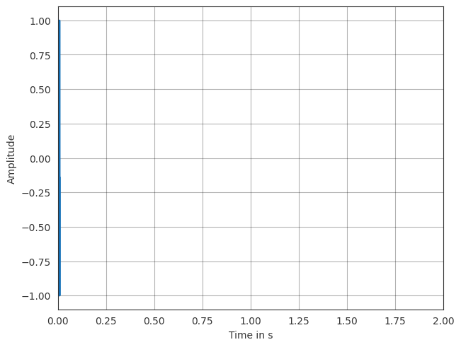
In many cases, the layout of the plot should be adjusted, which can be done using Matplotlib and the axes handle that is returned by all plot functions. For example, the range of the x-axis can be changed.
[16]:
ax = pf.plot.time(x_power)
ax.set_xlim(0, 2)
[16]:
(0.0, 2.0)
Note: For an easy use of the pyfar plotstyle (available as ‘light’ and ‘dark’ theme) wrappers for Matplotlib’s use and context are available as pyfar.plot.use and pyfar.plot.context.
Coordinates#
The Coordinates() class is designed for storing, manipulating, and accessing coordinate points. It supports a large variety of different coordinate conventions and the conversion between them. Examples for data that can be stored are microphone positions of a spherical microphone array and loudspeaker positions of a sound field synthesis system. Lets create an empty Coordinates object. Visit the coordinate
concepts for a graphical overview of this.
[17]:
c = pf.Coordinates()
Entering coordinate points#
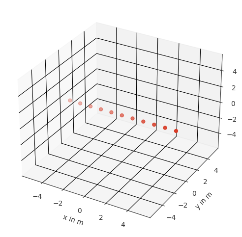
Coordinate points can be entered manually.
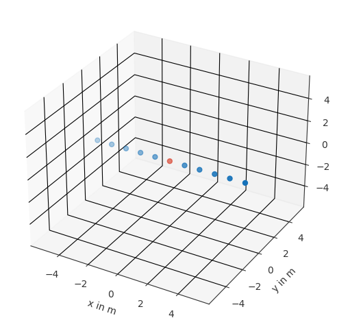
[18]:
c = pf.Coordinates(np.arange(-5., 6), 0, 0)
# show general information
print(c)
# plot the sampling points
c.show()
1D Coordinates object with 11 points of cshape (11,)
domain: cart, convention: right, unit: met
coordinates: x in meters, y in meters, z in meters
Does not contain sampling weights

Another way to initalize Coordinate objects is the pf.Coordinates(x, y, z) constructor or for other coordinate systems classmethods like pf.Coordinates.from_spherical_elevation(azimuth, elevation, radius). Visit the coordinate class for more datails.
[19]:
c1 = pf.Coordinates.from_spherical_elevation([0, np.pi/2, np.pi], 0, 1)
Inside the Coordinates object, the Coordinates are stored in a cartesian coordinate system for each x, y and z. Information about coordinate array can be obtained by c.cshape, c.csize, and c.cdim. These properties are similar to numpy’s shape, size, and dim of each x, y and z. Additionally we can use available sampling schemes contained in https://spharpy.readthedocs.io/en/latest/spharpy.samplings.html.
Retrieving coordinate points#
There are different ways to retrieve points from a Coordinates object. All points can be obtained in cartesian, spherical, and cylindrical coordinates using the related properties c.cartesian, c.sperical_evaluation and c.cylindrical. Also single properties of each coordinate system convention can be accessed by e.g. c.azimuth, c.radius or c.x. Visit the coordinate class for more details.”
[20]:
cartesian_coordinates = c.cartesian
Different methods are available for obtaining a specific subset of coordinates. For example, the nearest k point(s) can be obtained by
[21]:
find = pf.Coordinates.from_spherical_colatitude(270/180*np.pi, 90/180*np.pi, 1)
index_out, distance = c.find_nearest(find, k=1)
c.show(index_out)
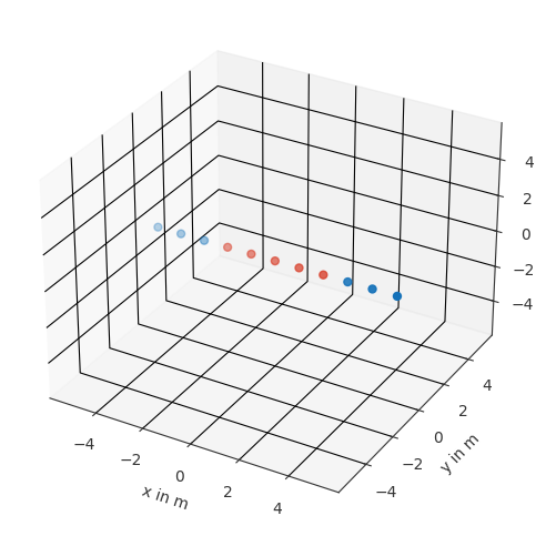
Another option is to find all points in a certain area around different points. Different distance measures are available.
[22]:
index_out = c.find_within(find, distance=3, distance_measure='euclidean')
c.show(index_out)
To obtain all points within a specified euclidean distance or arc distance, you can use c.get_nearest_cart() and c.get_nearest_sph(). To obtain more complicated subsets of any coordinate, e.g., the horizontal plane with colatitude=90 degree, you can use
[23]:
index_out = c.colatitude == 90/180*np.pi
c.show(index_out)
Rotating coordinates#
You can apply rotations using quaternions, rotation vectors/matrixes and euler angles with c.rotate(), which is a wrapper for scipy.spatial.transform.Rotation. For example rotating around the y-axis by 45 degrees can be done with
[24]:
c.rotate('y', 45)
c.show()
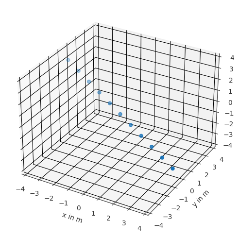
Note that this changes the points inside the Coordinates object, which means that you have to be careful not to apply the rotation multiple times, i.e., when evaluationg cells during debugging.
Orientations#
The Orientations() class is designed for storing, manipulating, and accessing orientation vectors. Examples for this are orientations of directional loudspeakers during measurements or head orientations. It is good to know that Orientations is inherited from scipy.spatial.transform.Rotation and that all methods of this class can also be used with Orientations.
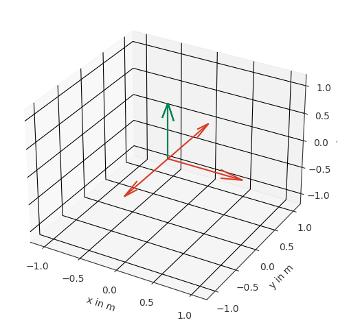
Entering orientations#
Lets go ahead and create an object and show the result
[25]:
views = [[0,  1, 0],
         [1,  0, 0],
         [0, -1, 0]]
up = [0, 0, 1]
orientations = pf.Orientations.from_view_up(views, up)
orientations.show(show_rights=False)
It is also possible to enter Orientations from Coordinates object or mixtures of Coordinates objects and array likes. This is equivalent to the example above
[26]:
azimuths = np.array([90, 0, 270]) * np.pi / 180
views_c = pf.Coordinates.from_spherical_elevation(azimuths, 0, 1)

orientations = pf.Orientations.from_view_up(views_c, up)
Retrieving orientations#
Orientaions can be retrieved as view, up, and right-vectors and in any format supported by scipy.spatial.transform.Rotation. They can also be converted into any coordinate convention supported by pyfar by putting them into a Coordinates object. Lets only check out one way for now
[27]:
views, ups, right, = orientations.as_view_up_right()
views
[27]:
array([[ 0.,  1.,  0.],
       [ 1.,  0.,  0.],
       [ 0., -1.,  0.]])
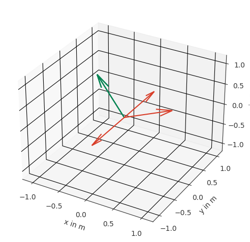
Rotating orientations#
Rotations can be done using the methods inherited from scipy.spatial.transform.Rotation. You can for example rotate around the y-axis this way
[28]:
rotation = pf.Orientations.from_euler('y', 30, degrees=True)
orientations_rot = orientations * rotation
orientations_rot.show(show_rights=False)
Signals#
The pyfar.signals module contains a variety of common audio signals including sine signals, sweeps, noise and pulsed noise. For brevity, lets have only one example
[29]:
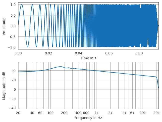
sweep = pf.signals.exponential_sweep_time(2**12, [100, 22050])
pf.plot.time_freq(sweep)
[29]:
array([<Axes: xlabel='Time in s', ylabel='Amplitude'>,
       <Axes: xlabel='Frequency in Hz', ylabel='Magnitude in dB'>],
      dtype=object)
DSP#
pyfar.dsp offers lots of useful functions to manipulate audio data including
convolution, deconvolution, and regulated inversion
windowing and zero-padding
generating linear and minimum phase signals
and many more. Have a look at the module documentation for a complete overview.
pyfar.dsp.filter contains wrappers for the most common filters of scipy.signal as well as more audio specific filter such as shelve and bell filters. Visit the filter types for an overview.
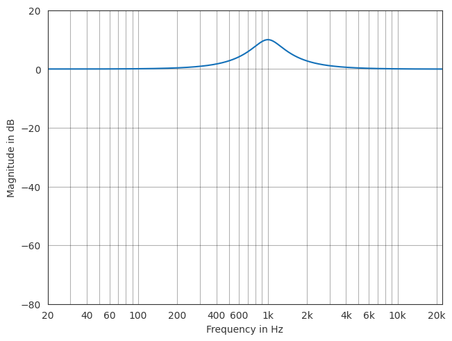
All filters can used in a similar manner, like this one
[30]:
x_filter = pf.dsp.filter.bell(x_energy, center_frequency=1e3, gain=10, quality=2)
pf.plot.line.freq(x_filter)
[30]:
<Axes: xlabel='Frequency in Hz', ylabel='Magnitude in dB'>
In’n’out#
Now that you know what pyfar is about, let’s see how you can save your work and read common data types.
Read and write pyfar data#
Pyfar contains functions for saving all pyfar objects and common data types such as numpy arrays using pf.io.write() and pf.io.read(). This creates .far files that also support compression.
Read and write audio-files#
Audio-files in wav or other formats are commonly used in the audio community to store and exchange data. You can read them with
signal = pf.io.read_audio(filename)
and write them with
pf.io.write_audio(signal, filename, overwrite=True).
You can write any signal to an audio, but in some cases, clipping will occur for values > 1. Multidimensional signals will be reshaped to 2D arrays before writing.
Read SOFA files#
SOFA files can be used to store spatially distributed acoustical data sets. Examples for this are room acoustic measurements at different positions in a room or a set of head-related transfer functions for different source positions. SOFA files can quickly be read by
signal, source, receiver = pf.io.read_sofa(filename)
which returns the audio data as a Signal or FrequencyData object (depending on the data in the SOFA file) and the source and receiver coordinates as a Coordinates object.
read_sofa uses the sofar package, which we recommend to manipulate and write SOFA files or access the detailed meta data contained in SOFA files.